Compute Transportable ROC Curve

Computes a receiver operating characteristic (ROC) curve in a target population using data transported from a source population. Returns sensitivity (TPR) and false positive rate (FPR) at multiple thresholds. Supports both counterfactual and factual prediction model transportability.

Usage

tr_roc(
  predictions,
  outcomes,
  treatment = NULL,
  source,
  covariates,
  treatment_level = NULL,
  analysis = c("transport", "joint"),
  estimator = c("dr", "om", "ipw", "naive"),
  selection_model = NULL,
  propensity_model = NULL,
  outcome_model = NULL,
  n_thresholds = 201,
  thresholds = NULL,
  include_naive = TRUE,
  ...
)

Arguments

predictions

Numeric vector of model predictions.

outcomes

Numeric vector of observed outcomes.

treatment

Numeric vector of treatment indicators (0/1), or NULL for factual prediction model transportability (no treatment/intervention). When NULL, only the selection model is used for weighting.

source

Numeric vector of population indicators (1=source/RCT, 0=target).

covariates

A matrix or data frame of baseline covariates.

treatment_level

The treatment level of interest (default: NULL). Required when treatment is provided; should be NULL when treatment is NULL (factual mode).

analysis

Character string specifying the type of analysis:

"transport": Use source outcomes for target estimation (default)
"joint": Pool source and target data

estimator

Character string specifying the estimator:

"naive": Naive estimator (biased)
"om": Outcome model estimator
"ipw": Inverse probability weighting estimator
"dr": Doubly robust estimator (default)

selection_model

Optional fitted selection model for P(S=0|X). If NULL, a logistic regression model is fit using the covariates.

propensity_model

Optional fitted propensity score model for P(A=1|X,S=1). If NULL, a logistic regression model is fit using source data.

outcome_model

Optional fitted outcome model for E[L(Y,g)|X,A,S]. If NULL, a regression model is fit using the relevant data. For binary outcomes, this should be a model for E[Y|X,A] (binomial family). For continuous outcomes, this should be a model for E[L|X,A] (gaussian family).

n_thresholds

Integer specifying the number of thresholds to evaluate. Thresholds are evenly spaced between 0 and 1. Default is 201.

thresholds

Optional numeric vector of specific thresholds to use. If provided, overrides n_thresholds.

include_naive

Logical indicating whether to also compute the naive ROC curve for comparison. Default is TRUE.

...

Additional arguments passed to internal functions.

Value

An object of class c("tr_roc", "roc_curve") containing:

thresholds: Thresholds used
sensitivity: Sensitivity (TPR) at each threshold
fpr: False positive rate at each threshold
specificity: Specificity at each threshold
naive_sensitivity: Naive sensitivity (if include_naive=TRUE)
naive_fpr: Naive FPR (if include_naive=TRUE)
auc: Area under the ROC curve (computed via trapezoidal rule)
naive_auc: Naive AUC (if include_naive=TRUE)
estimator: Estimator used
analysis: Analysis type
n_source: Number of source observations
n_target: Number of target observations
treatment_level: Treatment level (NULL for factual mode)

Details

The ROC curve plots sensitivity (true positive rate) against the false positive rate (1 - specificity) at various classification thresholds.

Counterfactual Mode (treatment provided)

When treatment is specified, computes the ROC curve for counterfactual outcomes under a hypothetical intervention.

Factual Mode (treatment = NULL)

When treatment is NULL, computes the ROC curve for observed outcomes in the target population using inverse-odds weighting based on the selection model only.

This function computes transportable sensitivity and FPR at multiple thresholds using the estimators from tr_sensitivity() and tr_fpr(). The area under the curve (AUC) is computed using the trapezoidal rule on the discrete threshold grid. For exact AUC estimation, use tr_auc() which employs the Wilcoxon-Mann-Whitney statistic.

For efficient computation, all thresholds are evaluated in a single pass through the data, with nuisance models fitted only once.

References

Steingrimsson, J. A., et al. (2023). "Transporting a Prediction Model for Use in a New Target Population." American Journal of Epidemiology, 192(2), 296-304. doi:10.1093/aje/kwac128

Steingrimsson, J. A., Wen, L., Voter, S., & Dahabreh, I. J. (2024). "Interpretable meta-analysis of model or marker performance." arXiv preprint arXiv:2409.13458.

Examples

# Generate example data
set.seed(123)
n <- 500
x <- rnorm(n)
s <- rbinom(n, 1, plogis(0.5 - 0.3 * x))
a <- ifelse(s == 1, rbinom(n, 1, 0.5), rbinom(n, 1, plogis(-0.5 + 0.5 * x)))
y <- rbinom(n, 1, plogis(-1 + x - 0.5 * a))
pred <- plogis(-1 + 0.8 * x)

# Compute transportable ROC curve
roc <- tr_roc(
  predictions = pred,
  outcomes = y,
  treatment = a,
  source = s,
  covariates = data.frame(x = x),
  n_thresholds = 51
)
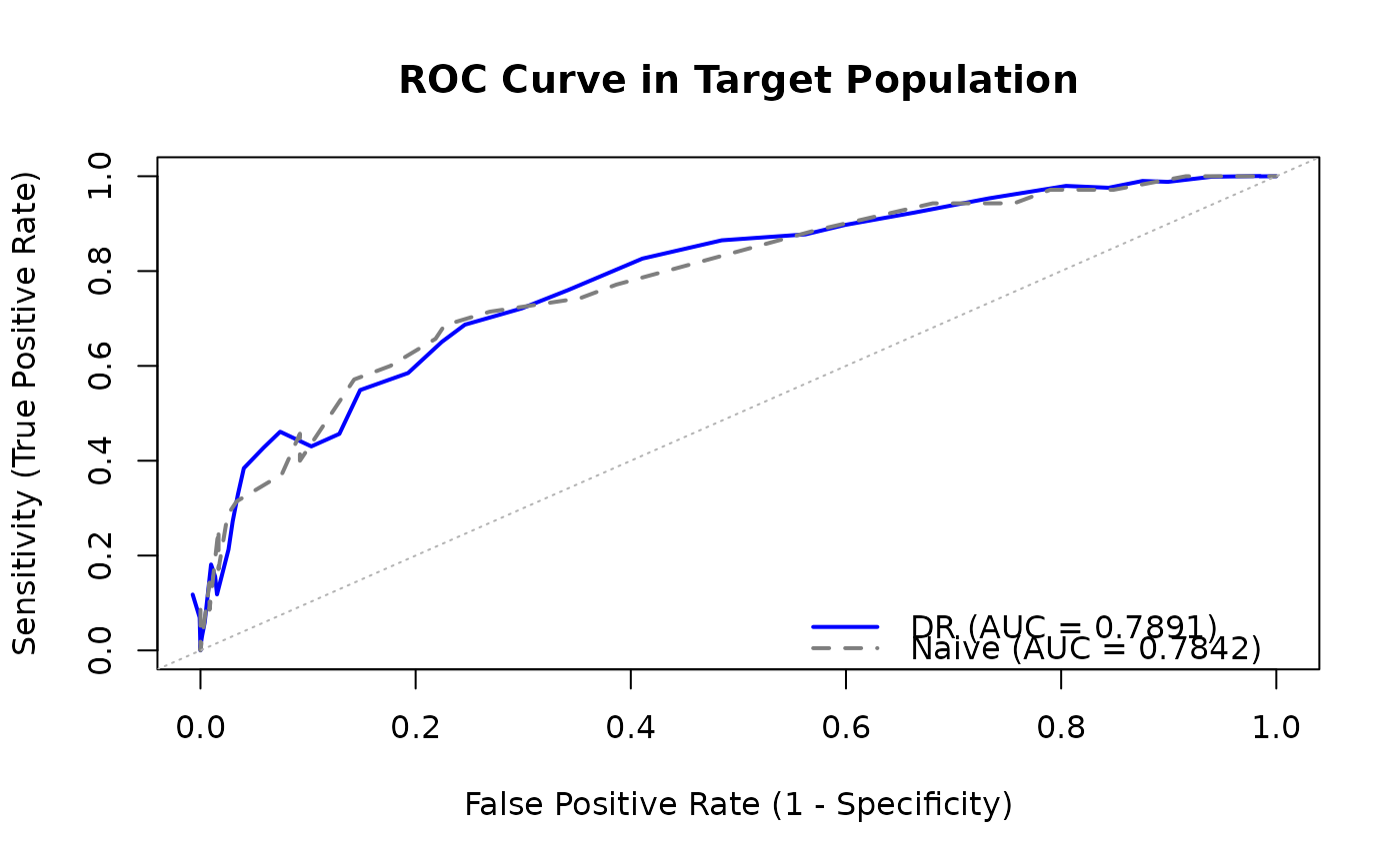
print(roc)
#> 
#> Transportable ROC Curve
#> =======================
#> 
#> Estimator: DR 
#> Analysis: transport 
#> Treatment level: 1 
#> N (source): 309 
#> N (target): 191 
#> Thresholds evaluated: 51 
#> 
#> AUC: 0.7891 
#> Naive AUC: 0.7842 
#> 
#> Use plot() to visualize the ROC curve.
#> 

# Plot the ROC curve
plot(roc)