Introduction to cfperformance

Overview

The cfperformance package provides methods for estimating prediction model performance under hypothetical (counterfactual) interventions. This is essential when:

Prediction models will be deployed in settings where treatment policies differ from training - A model trained on patients who received a mixture of treatments may perform differently when deployed where everyone receives a specific treatment.
Predictions support treatment decisions - When predictions inform who should receive treatment, naive performance estimates conflate model accuracy with treatment effects.

The methods implemented here are based on Boyer, Dahabreh & Steingrimsson (2025), “Estimating and evaluating counterfactual prediction models,” Statistics in Medicine, 44(23-24), e70287. doi:10.1002/sim.70287

Installation

# Install from GitHub
# install.packages("devtools")
devtools::install_github("boyercb/cfperformance")

Quick Start

# Load the included example dataset
data(cvd_sim)
head(cvd_sim)
#>          age          bp       chol treatment event risk_score
#> 1 -0.2078913 -0.43879526 -0.5697974         0     0 0.07548152
#> 2 -1.2517361  1.30171507  0.7798967         0     0 0.13491154
#> 3  1.7957878 -0.39076092 -0.1731313         1     0 0.18333022
#> 4 -1.2464064  0.08506276  0.0269594         1     0 0.07145644
#> 5 -0.5880067  0.10358176  0.8346190         1     0 0.11730651
#> 6 -0.9132198  0.88158838  0.6061392         0     0 0.12684642

The cvd_sim dataset contains simulated cardiovascular data with:

age, bp, chol: Patient covariates
treatment: Binary treatment indicator (confounded by covariates)
event: Binary outcome (cardiovascular event)
risk_score: Pre-computed predictions from a logistic regression model

Estimating Counterfactual MSE

Now we can estimate how well the model would perform if everyone were untreated (treatment_level = 0):

# Estimate MSE under counterfactual "no treatment" policy
mse_result <- cf_mse(
  predictions = cvd_sim$risk_score,
  outcomes = cvd_sim$event,
  treatment = cvd_sim$treatment,
  covariates = cvd_sim[, c("age", "bp", "chol")],
  treatment_level = 0,
  estimator = "dr"  # doubly robust estimator
)

mse_result
#> 
#> Counterfactual MSE Estimation
#> ---------------------------------------- 
#> Estimator: dr 
#> Treatment level: 0 
#> N observations: 2500 
#> 
#> Estimate: 0.1186 (SE: 0.0062 )
#> 95% CI: [0.1072, 0.1303]
#> 
#> Naive estimate: 0.1086

The doubly robust estimator adjusts for confounding using both a propensity score model and an outcome model, providing consistent estimates even if one model is misspecified.

Comparing Estimators

Let’s compare all available estimators:

estimators <- c("naive", "cl", "ipw", "dr")
results <- sapply(estimators, function(est) {
  cf_mse(
    predictions = cvd_sim$risk_score,
    outcomes = cvd_sim$event,
    treatment = cvd_sim$treatment,
    covariates = cvd_sim[, c("age", "bp", "chol")],
    treatment_level = 0,
    estimator = est
  )$estimate
})
names(results) <- estimators
round(results, 4)
#>  naive     cl    ipw     dr 
#> 0.1086 0.1190 0.1192 0.1186

naive: Simply computes MSE on the subset with the target treatment level. Biased when treatment is confounded.
cl (Conditional Loss): Models the outcome and integrates over the covariate distribution.
ipw (Inverse Probability Weighting): Reweights observations to mimic the counterfactual population.
dr (Doubly Robust): Combines outcome modeling and IPW; consistent if either model is correct.

Estimating Counterfactual AUC

For discrimination (AUC), we can use similar methods:

auc_result <- cf_auc(
  predictions = cvd_sim$risk_score,
  outcomes = cvd_sim$event,
  treatment = cvd_sim$treatment,
  covariates = cvd_sim[, c("age", "bp", "chol")],
  treatment_level = 0,
  estimator = "dr"
)

auc_result
#> 
#> Counterfactual AUC Estimation
#> ---------------------------------------- 
#> Estimator: dr 
#> Treatment level: 0 
#> N observations: 2500 
#> 
#> Estimate: 0.682 (SE: 0.0209 )
#> 95% CI: [0.6444, 0.725]
#> 
#> Naive estimate: 0.6729

ROC Curve

We can also visualize the full ROC curve, which shows the tradeoff between sensitivity (true positive rate) and 1-specificity (false positive rate) across all classification thresholds:

roc_result <- cf_roc(
  predictions = cvd_sim$risk_score,
  outcomes = cvd_sim$event,
  treatment = cvd_sim$treatment,
  covariates = cvd_sim[, c("age", "bp", "chol")],
  treatment_level = 0,
  estimator = "dr",
  include_naive = TRUE
)

# Plot the ROC curve
plot(roc_result)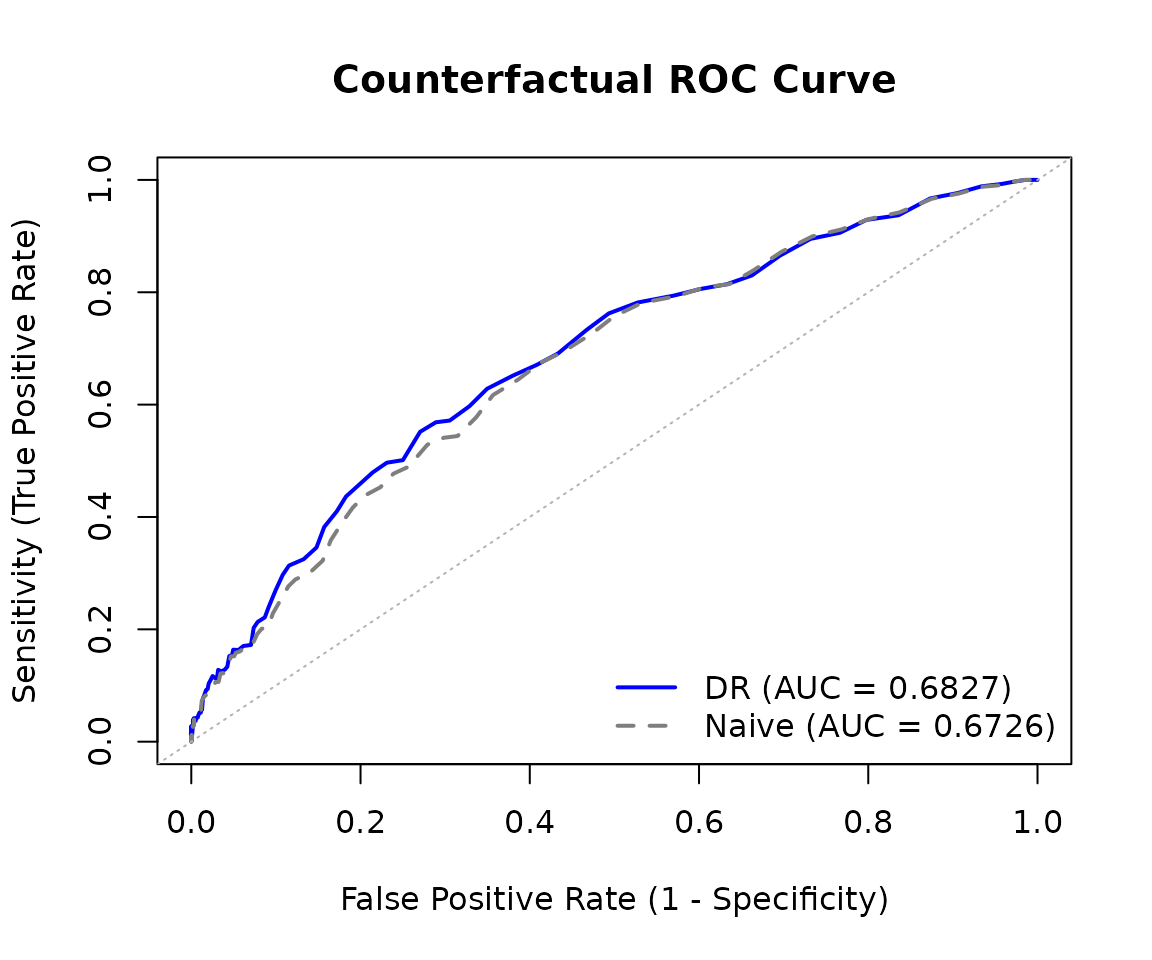

The ROC curve data can also be extracted as a data frame for custom plotting:

roc_df <- as.data.frame(roc_result)
head(roc_df)
#>   threshold       fpr sensitivity  specificity     type
#> 1     0.000 1.0000000    1.000000 0.0000000000 adjusted
#> 2     0.005 1.0000000    1.000000 0.0000000000 adjusted
#> 3     0.010 1.0000000    1.000000 0.0000000000 adjusted
#> 4     0.015 0.9990597    1.000008 0.0009403139 adjusted
#> 5     0.020 0.9985887    1.000017 0.0014112567 adjusted
#> 6     0.025 0.9957604    1.000083 0.0042395558 adjusted

Bootstrap Standard Errors

Both functions support bootstrap standard errors:

mse_with_se <- cf_mse(
  predictions = cvd_sim$risk_score,
  outcomes = cvd_sim$event,
  treatment = cvd_sim$treatment,
  covariates = cvd_sim[, c("age", "bp", "chol")],
  treatment_level = 0,
  estimator = "dr",
  se_method = "bootstrap",
  n_boot = 200
)
mse_with_se
#> 
#> Counterfactual MSE Estimation
#> ---------------------------------------- 
#> Estimator: dr 
#> Treatment level: 0 
#> N observations: 2500 
#> 
#> Estimate: 0.1186 (SE: 0.0064 )
#> 95% CI: [0.1068, 0.1317]
#> 
#> Naive estimate: 0.1086

Calibration Curves

The package also supports counterfactual calibration assessment:

cal_result <- cf_calibration(
  predictions = cvd_sim$risk_score,
  outcomes = cvd_sim$event,
  treatment = cvd_sim$treatment,
  covariates = cvd_sim[, c("age", "bp", "chol")],
  treatment_level = 0
)

# Plot calibration curve
plot(cal_result)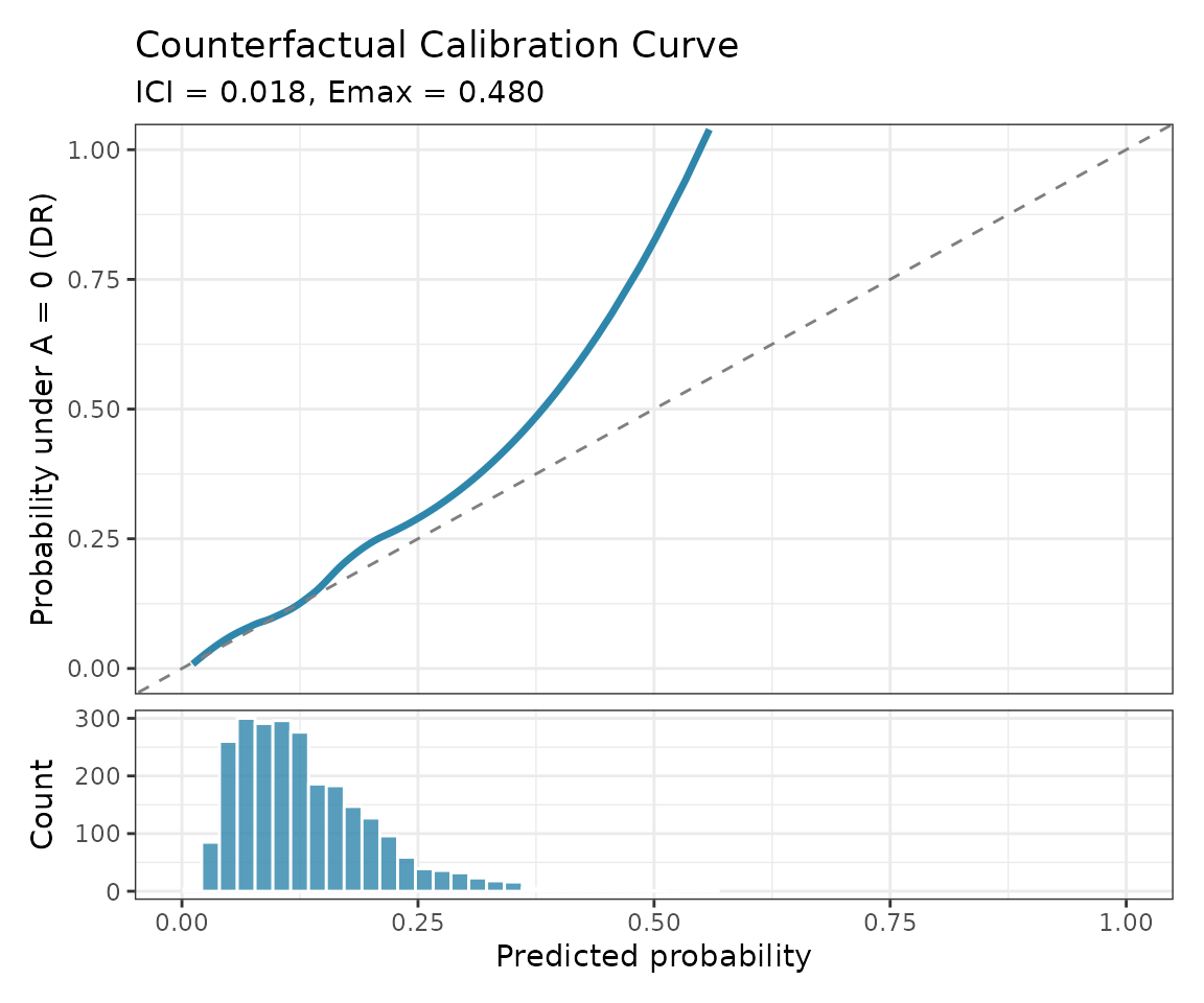

Cross-Validation for Model Selection

When comparing multiple prediction models, use counterfactual cross-validation:

# Compare two models using counterfactual CV
models <- list(
  "Simple" = event ~ age,
  "Full" = event ~ age + bp + chol
)

comparison <- cf_compare(
  models = models,
  data = cvd_sim,
  treatment = "treatment",
  treatment_level = 0,
  metric = "mse",
  K = 5
)

comparison
#> 
#> Counterfactual Model Comparison
#> --------------------------------------------- 
#> Method: cv (K = 5 )
#> Estimator: dr 
#> 
#>   model mse_mean mse_se mse_naive_mean
#>  Simple   0.1236 0.0061      0.1122797
#>    Full   0.1185 0.0017      0.1088334
#> 
#> Best model: Full

Key Concepts

Why Counterfactual Performance?

Standard model performance evaluation computes metrics like MSE or AUC on a test set. However, this answers: “How well does the model predict outcomes as they occurred?”

When a model will be used to inform treatment decisions, we often need to answer: “How well would the model predict outcomes if everyone received (or didn’t receive) treatment?”

These can differ substantially when:

Treatment is related to the outcome (treatment effects exist)
Treatment is related to the covariates used for prediction (confounding)

Assumptions

The methods in this package require:

Consistency: Observed outcomes equal potential outcomes under the observed treatment.
Positivity: All covariate patterns have positive probability of receiving each treatment level.
No unmeasured confounding: Treatment is independent of potential outcomes given measured covariates.

These are standard causal inference assumptions. The package provides warnings when positivity may be violated (extreme propensity scores).

Choosing an Estimator

Use doubly robust (dr) as the default - it’s consistent if either the propensity or outcome model is correct.
Use ipw when you trust your propensity model but not your outcome model.
Use cl when you trust your outcome model but not your propensity model.
Use naive only as a baseline comparison.

Christopher Boyer, Issa Dahabreh, Jon Steingrimsson

2026-01-28