Transportability Analysis with cfperformance

Overview

This vignette demonstrates how to use the transportability functions in cfperformance to evaluate prediction model performance when transporting from a source population (such as a randomized controlled trial) to a target population.

The methods are based on Voter et al. (2025), “Transportability of machine learning-based counterfactual prediction models with application to CASS,” Diagnostic and Prognostic Research, 9(4). doi:10.1186/s41512-025-00201-y

When to Use Transportability Analysis

Transportability analysis is appropriate when:

You have a prediction model trained in one population (e.g., an RCT)
You want to evaluate performance in a different target population
Treatment is randomized in the source population
Covariates are measured in both populations

Common scenarios include:

Evaluating an RCT-derived risk score in a real-world patient population
Assessing whether a clinical prediction rule “transports” to a new setting
Understanding how model performance varies across populations

The Setting

Consider two populations:

Source (S=1): Often an RCT where treatment A is randomized
Target (S=0): The population where we want to deploy the model

We observe: - Covariates X in both populations - Treatment A in both populations
- Outcomes Y in the source (and possibly target) - Model predictions g(X) for all individuals

The goal is to estimate the counterfactual prediction performance $E[L(Y^a, g(X)) | S=0]$ — how well would the model perform in the target population if everyone received treatment level a?

Using the Included Example Data

The package includes a simulated transportability dataset:

data(transport_sim)
head(transport_sim)
#>           age   biomarker smoking source treatment event risk_score
#> 1  0.63916439 -0.06780891       1      1         0     0  0.3388230
#> 2  0.06014812  0.81999552       0      1         0     0  0.3309058
#> 3  0.78997359 -1.00222911       1      0         1     0  0.2773807
#> 4  1.28410328  0.78155960       1      0         1     0  0.4481046
#> 5  0.39198673  1.24382106       0      1         1     0  0.3841622
#> 6 -0.13627856  0.61176294       1      1         1     0  0.3482827

# Population sizes
cat("Source (RCT) n =", sum(transport_sim$source == 1), "\n")
#> Source (RCT) n = 1276
cat("Target n =", sum(transport_sim$source == 0), "\n")
#> Target n = 1224

The transport_sim dataset contains: - age, biomarker, smoking: Patient covariates - source: Population indicator (1 = source/RCT, 0 = target) - treatment: Binary treatment (randomized in source, confounded in target) - event: Binary outcome - risk_score: Predictions from a model trained in the source population

Transport Analysis

The transport analysis uses outcomes from the source/RCT to estimate performance in the target population. This is useful when:

Outcomes are only observed in the RCT
You want to leverage randomization in the source

MSE in the Target Population

mse_result <- tr_mse(
  predictions = transport_sim$risk_score,
  outcomes = transport_sim$event,
  treatment = transport_sim$treatment,
  source = transport_sim$source,
  covariates = transport_sim[, c("age", "biomarker", "smoking")],
  treatment_level = 0,  # Evaluate under no treatment
  analysis = "transport",
  estimator = "dr",
  se_method = "none"
)

print(mse_result)
#> 
#> Counterfactual Transportable MSE Estimation
#> --------------------------------------------- 
#> Analysis: transport 
#> Estimator: dr 
#> Treatment level: 0 
#> N target: 1224  | N source: 1276 
#> 
#> Estimate: 0.2219
#> 
#> Naive estimate: 0.2178

Comparing Estimators

Let’s compare all four estimators:

estimators <- c("naive", "om", "ipw", "dr")

mse_estimates <- sapply(estimators, function(est) {
  result <- tr_mse(
    predictions = transport_sim$risk_score,
    outcomes = transport_sim$event,
    treatment = transport_sim$treatment,
    source = transport_sim$source,
    covariates = transport_sim[, c("age", "biomarker", "smoking")],
    treatment_level = 0,
    analysis = "transport",
    estimator = est,
    se_method = "none"
  )
  result$estimate
})

data.frame(
  Estimator = estimators,
  MSE = round(mse_estimates, 4)
)
#>       Estimator    MSE
#> naive     naive 0.2178
#> om           om 0.2222
#> ipw         ipw 0.2213
#> dr           dr 0.2219

naive: Uses source data with A=0 only (ignores population differences)
om (outcome model): Models E[L|X,A,S=1] and averages over target X
ipw: Reweights source observations to match target population
dr (doubly robust): Combines outcome modeling and IPW

AUC in the Target Population

For discrimination, we can estimate the transportable AUC:

auc_result <- tr_auc(
  predictions = transport_sim$risk_score,
  outcomes = transport_sim$event,
  treatment = transport_sim$treatment,
  source = transport_sim$source,
  covariates = transport_sim[, c("age", "biomarker", "smoking")],
  treatment_level = 0,
  analysis = "transport",
  estimator = "dr",
  se_method = "none"
)

print(auc_result)
#> 
#> Counterfactual Transportable AUC Estimation
#> --------------------------------------------- 
#> Analysis: transport 
#> Estimator: dr 
#> Treatment level: 0 
#> N target: 1224  | N source: 1276 
#> 
#> Estimate: 0.6204
#> 
#> Naive estimate: 0.6249

ROC Curve in the Target Population

We can visualize the full ROC curve for the target population:

roc_result <- tr_roc(
  predictions = transport_sim$risk_score,
  outcomes = transport_sim$event,
  treatment = transport_sim$treatment,
  source = transport_sim$source,
  covariates = transport_sim[, c("age", "biomarker", "smoking")],
  treatment_level = 0,
  analysis = "transport",
  estimator = "dr",
  include_naive = TRUE
)

# Plot the ROC curve
plot(roc_result)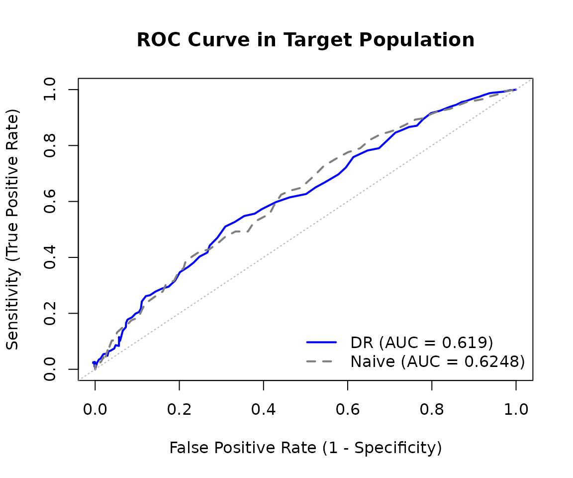

The comparison between the doubly robust and naive ROC curves shows how performance estimates change when properly accounting for the distribution shift between source and target populations.

Calibration in the Target Population

To assess calibration in the target population:

calib_result <- tr_calibration(
  predictions = transport_sim$risk_score,
  outcomes = transport_sim$event,
  treatment = transport_sim$treatment,
  source = transport_sim$source,
  covariates = transport_sim[, c("age", "biomarker", "smoking")],
  treatment_level = 0,
  analysis = "transport",
  estimator = "ipw",
  smoother = "loess",
  se_method = "none"
)

print(calib_result)
#> 
#> Counterfactual Transportable CALIBRATION Estimation
#> --------------------------------------------- 
#> Analysis: transport 
#> Estimator: ipw 
#> Treatment level: 0 
#> N target: 1224  | N source: 1276 
#> 
#> Calibration Metrics:
#>   ICI (Integrated Calibration Index): 0.0546 
#>   E50 (Median absolute error): 0.0558 
#>   E90 (90th percentile error): 0.0852 
#>   Emax (Maximum error): 0.1806

plot(calib_result)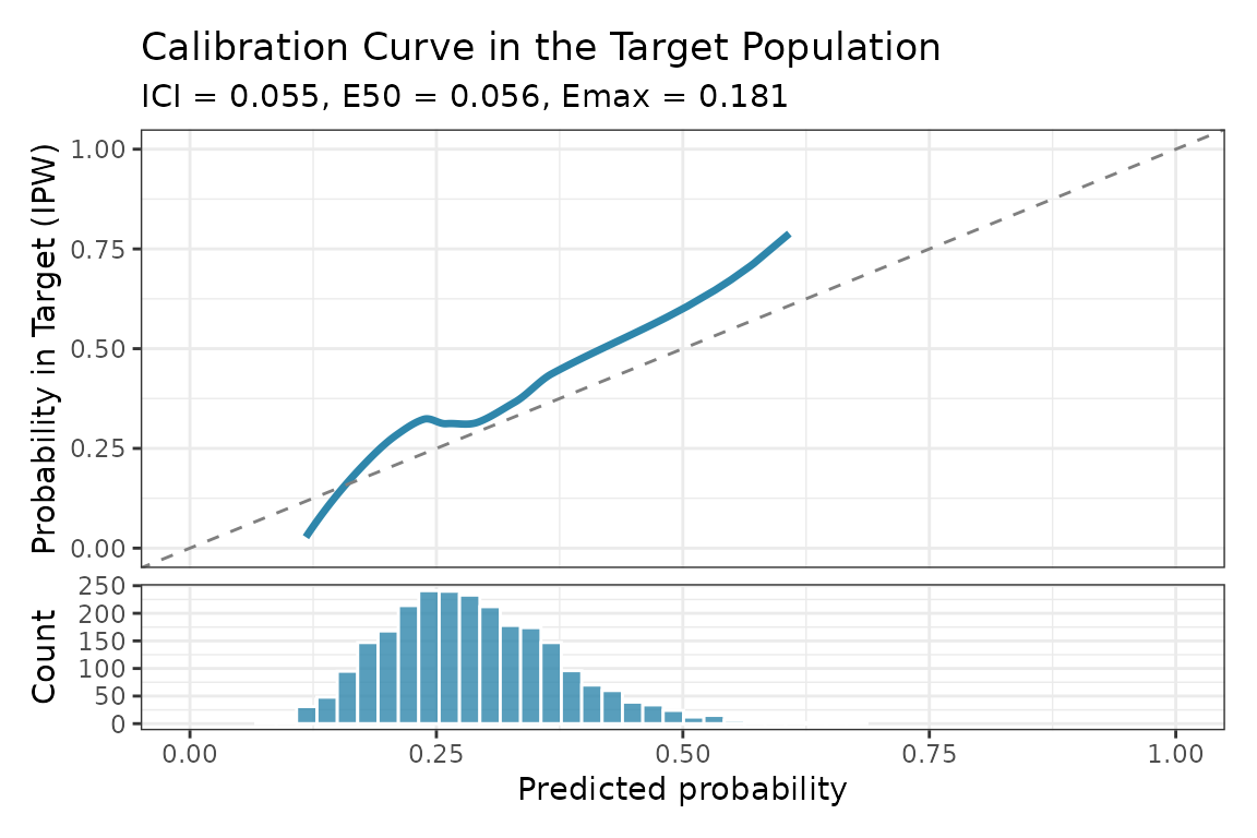

Transportable calibration curve for the target population

Joint Analysis

The joint analysis pools source and target data for potentially more efficient estimation. This requires outcome data in both populations.

mse_joint <- tr_mse(
  predictions = transport_sim$risk_score,
  outcomes = transport_sim$event,
  treatment = transport_sim$treatment,
  source = transport_sim$source,
  covariates = transport_sim[, c("age", "biomarker", "smoking")],
  treatment_level = 0,
  analysis = "joint",  # Pool data
  estimator = "dr",
  se_method = "none"
)

cat("Transport MSE:", round(mse_result$estimate, 4), "\n")
#> Transport MSE: 0.2219
cat("Joint MSE:", round(mse_joint$estimate, 4), "\n")
#> Joint MSE: 0.2223

Factual Prediction Model Transportability

The examples above use counterfactual transportability, which estimates performance under a hypothetical treatment intervention. However, many prediction models are developed without a causal/counterfactual interpretation.

For factual prediction model transportability — estimating how well a model predicts observed outcomes in the target population — you can omit the treatment and treatment_level arguments:

# Factual transportability (no treatment/intervention)
mse_factual <- tr_mse(
  predictions = transport_sim$risk_score,
  outcomes = transport_sim$event,
  source = transport_sim$source,
  covariates = transport_sim[, c("age", "biomarker", "smoking")],
  # treatment = NULL (default),
  # treatment_level = NULL (default),
  analysis = "transport",
  estimator = "dr",
  se_method = "none"
)

print(mse_factual)
#> 
#> Factual Transportable MSE Estimation
#> --------------------------------------------- 
#> Analysis: transport 
#> Estimator: dr 
#> N target: 1224  | N source: 1276 
#> 
#> Estimate: 0.1892
#> 
#> Naive estimate: 0.1948

Notice the output shows “Factual Transportable” to indicate this mode.

Factual vs Counterfactual Mode

Factual mode (treatment = NULL):

Estimates E[L(Y, g(X)) | S=0] — performance on observed outcomes
Uses only the selection model P(S=0|X) for inverse-odds weighting
No propensity score model needed
Appropriate for standard prediction models without causal interpretation

Counterfactual mode (treatment provided):

Estimates E[L(Y^a, g(X)) | S=0] — performance on counterfactual outcomes
Uses both selection model P(S=0|X) and propensity model P(A=a|X, S=1)
Appropriate when the prediction target is a counterfactual outcome

Factual Transportability for AUC and Other Metrics

All tr_* functions support factual mode:

# Factual AUC
auc_factual <- tr_auc(
  predictions = transport_sim$risk_score,
  outcomes = transport_sim$event,
  source = transport_sim$source,
  covariates = transport_sim[, c("age", "biomarker", "smoking")],
  analysis = "transport",
  estimator = "dr",
  se_method = "none"
)

print(auc_factual)
#> 
#> Factual Transportable AUC Estimation
#> --------------------------------------------- 
#> Analysis: transport 
#> Estimator: dr 
#> N target: 1224  | N source: 1276 
#> 
#> Estimate: 0.6009
#> 
#> Naive estimate: 0.6126

# Factual sensitivity at threshold 0.3
sens_factual <- tr_sensitivity(
  predictions = transport_sim$risk_score,
  outcomes = transport_sim$event,
  source = transport_sim$source,
  covariates = transport_sim[, c("age", "biomarker", "smoking")],
  threshold = 0.3,
  analysis = "transport",
  estimator = "dr",
  se_method = "none"
)

print(sens_factual)
#> 
#> Factual Transportable Sensitivity Estimate
#> ===================================
#> 
#> Estimator: DR 
#> Analysis: transport 
#> N (source): 1276 
#> N (target): 1224 
#> 
#> Threshold: 0.3 
#> Estimate: 0.5573 
#> Naive estimate: 0.4538

References for Factual Transportability

The factual transportability approach is based on:

Steingrimsson, J. A., et al. (2023). “Transporting a Prediction Model for Use in a New Target Population.” American Journal of Epidemiology, 192(2), 296-304. doi:10.1093/aje/kwac128

Li, S., et al. (2023). “Efficient estimation of the expected prediction error under covariate shift.” Biometrics, 79(1), 295-307. doi:10.1111/biom.13583

Bootstrap Standard Errors

For inference, use bootstrap standard errors:

mse_with_se <- tr_mse(
  predictions = transport_sim$risk_score,
  outcomes = transport_sim$event,
  treatment = transport_sim$treatment,
  source = transport_sim$source,
  covariates = transport_sim[, c("age", "biomarker", "smoking")],
  treatment_level = 0,
  analysis = "transport",
  estimator = "dr",
  se_method = "bootstrap",
  n_boot = 500,
  stratified_boot = TRUE  # Preserve source/target ratio
)

summary(mse_with_se)
#> 
#> Summary: Counterfactual Transportable MSE Estimation
#> ======================================================= 
#> 
#> Call:
#> tr_mse(predictions = transport_sim$risk_score, outcomes = transport_sim$event, 
#>     treatment = transport_sim$treatment, source = transport_sim$source, 
#>     covariates = transport_sim[, c("age", "biomarker", "smoking")], 
#>     treatment_level = 0, analysis = "transport", estimator = "dr", 
#>     se_method = "bootstrap", n_boot = 500, stratified_boot = TRUE)
#> 
#> Settings:
#>   Mode: Counterfactual 
#>   Analysis type: transport 
#>   Estimator: dr 
#>   Treatment level: 0 
#>   Target sample size: 1224 
#>   Source sample size: 1276 
#> 
#> Results:
#>      Estimator Estimate       SE CI_lower CI_upper
#>  Transportable   0.2219 0.008787   0.2055   0.2404
#>          Naive   0.2178       NA       NA       NA
#> 
#> Difference (Transportable - Naive): 0.0041
confint(mse_with_se)
#>            2.5%     97.5%
#> tr_mse 0.205452 0.2403893

The stratified_boot = TRUE option (default) ensures that bootstrap samples preserve the ratio of source to target observations, which is recommended for transportability analysis.

Key Assumptions

The transportability estimators rely on several assumptions:

1. Consistency in the Source and Target Populations.

For all individuals $i$ , we have $Y_i^a = Y_i$ if $A_i = a$ .

The observed outcome equals the potential outcome under the received treatment. Implies no interference and well-defined treatments.

2. Conditional Exchangeability in the Source Population (Trial)

$(Y^a \perp A) | X, S=1$

Treatment is randomized in the source population, so there is no confounding between treatment and outcome given covariates.

3. Positivity of Treatment in the Source Population (Trial)

$P(A=a|X, S=1) > 0 \text{ for the treatment level of interest}$

In the source population, the treatment level must have positive probability (guaranteed by randomization).

4. Conditional Exchangeability (Transportability)

$(Y^a \perp S) | X$

The potential outcome is independent of population membership given covariates. This means the source population is “representative” of how the outcome model would perform in the target, after conditioning on X.

5. Positivity of Selection

$P(S=0|X) > 0 \text{ and } P(S=1|X) > 0 \text{ for all } X$

Both populations must have positive probability for all covariate values.

When to Use Each Function

Scenario	Function	Analysis
Single population, observational data	`cf_mse()`, `cf_auc()`, `cf_calibration()`	-
Source (RCT) to target, outcomes in source only	`tr_mse()`, `tr_auc()`, `tr_calibration()`	`"transport"`
Source + target, outcomes in both	`tr_mse()`, `tr_auc()`, `tr_calibration()`	`"joint"`

Comparison with cf_* Functions

The cf_* functions (counterfactual) are for single-population analysis:

Use observational data from one population
Adjust for confounding between treatment and outcome
Equivalent to “Observational (OBS)” estimators in Voter et al.

The tr_* functions (transportability) are for two-population analysis:

Transport from source to target population
Leverage randomization in source (if RCT)
Adjust for differences in covariate distributions

References

Voter, S. R., et al. (2025). “Transportability of machine learning-based counterfactual prediction models with application to CASS.” Diagnostic and Prognostic Research, 9(4). doi:10.1186/s41512-025-00201-y

Boyer, C. B., Dahabreh, I. J., & Steingrimsson, J. A. (2025). “Estimating and evaluating counterfactual prediction models.” Statistics in Medicine, 44(23-24), e70287. doi:10.1002/sim.70287